Modelling of strongly lensed galaxies in the uv plane

In sub-mm/mm selected gravitational lensing events the background source is usually a dusty star forming galaxy (DSFG) at redshift z > 1. Because of dust obscuration and distance, the lensed DSFG is very faint at optical/near-infrared wavelengths, and in general overcame by the emission from the foreground object that acts as the lens, typically a massive elliptical galaxy. Therefore, in order to reveal the multiple images of the lensed DSFG and to get data usable for lens modelling and source reconstruction, it is crucial to obtain high spatial resolution (i.e. sub-arcsecond) follow-up observations directly at sub-mm/mm wavelengths, where the background source is the brightest and the contamination from the lens is negligible.

Unfortunately, as observations are carried out at longer wavelengths the resolution is worsened due to the diffraction limit of the telescope:

(1) $\begin{equation*} \theta = 1.22 \frac{\lambda}{D}, \end{equation*}$

where $\theta$ is the minimum separation at which tow point source can still be distinguished, $D$ is the diameter of the telescope and $\lambda$ is the wavelength of observations.

Figure 1. Comparing the spatial resolution of Hubble and Herschel.

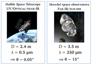
An example of this effect is illustrated in Fig. 1, where I compare the performance of the Hubble Space Telescope (HST) and of the Herschel Space Observatory. The latter has a 3.5m diameter mirror, bigger than the 2.4m diameter mirror of HST. However Herschel explored the Universe at wavelengths that are hundreds of times longer than those observed by the HST. So, despite the wider mirror, Herschel could not resolve anything below ~10″, while HST can produce very sharp images in the optical.

One might think of overcoming this problem by simply building a larger telescope. Unfortunately, if you do your maths, by using the diffraction limit formula, you will find that you need to erect an antenna of 10km in diameter to produce HST-quality images at sub-millimeter wavelengths, which is clearly not feasible! But no need to despair! Sub-arcsecond spatial resolutions can still be achieved at sub-mm/mm/radio wavelengths using a trick. This trick is called interferometry.

Interferometry

An interferometer is an array of antennas which work all together by correlating their signals. In doing so they can mimic the performance of a much larger telescope. Not all the antennas are fixed in the ground but at least some of them are movable and can be separated by large distances, or baselines, of up to several kilometers. The larger the separation the higher the resolution that can be achieved: in a nutshell, the baseline corresponds to the diameter of the theoretical telescope that the interferometer is trying to mimic.

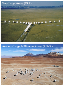
Figure 2. Example of interferometers: the VLA, in New Mexico, and the ALMA, in the Chilean desert of Atacama

The Very Large Array (VLA), in New-Mexico (USA) and the Atacama Large Millimeter Array (ALMA), in Chile, shown in Fig. 2, are examples of interferometers. They operate at radio and sub-mm/mm wavelengths, respectively, and can achieve spatial resolutions of the order to few tens of milliarcseconds! Very impressive indeed!

Of course, there is a drawback. No matter how many antennas the interferometer comprises, they will never manage to fill the entire area of the theoretical big telescope. This has inevitably an impact on the quality of the images, as I will show you next.

An interferometer does not directly measure the surface brightness of the source, but, instead, it samples its Fourier transform.

By correlating the signal of the astrophysical source collected by the array of antennas the interferometer produces the visibility function, $V(u,v)$ , that is the Fourier transform of the source surface brightness, $I(x,y)$ , sampled at a finite number of locations in the Fourier space, or $uv$ -plane:

(2) $\begin{equation*} V(u,v) = \int\int A(x,y)I(x,y)e^{-2\pi i (ux + vy)} dxdy, \end{equation*}$

where $A$ is the effective collecting area of each antenna, i.e. the primary beam.

The source surface brightness, weighted by the primary beam, is then obtained via an anti-Fourier transform

(3) $\begin{equation*} A(x,y)I(x,y) = \int\int V(u,v)e^{2\pi i (ux + vy)} dudv \end{equation*}$

In Fig. 3 I show the simulated interferometric observations of the model lensed galaxy discussed in Modelling of strongly lensed galaxies. I have used the simobserve and simanalysize tasks in the Common Astronomy Software Application (CASA) package to produce the figure. The righ-hand panel gives you an idea of the data provided by the interferometer, i.e. a finite number of data points distributed over the $uv$ -plane. Once you anti-Fourier transform them you get the image of the astronomical source, shown in the right-hand panel of Fig. 3. You may appreciate the presence of substructures in the image: most of it is not real but is just a consequence of the finite sampling of the $uv$ -plane, of the antennas configuration and of correlated noise.

Figure 3. Simulation of ALMA observations. *Left-hand panel*: sampling of the uv-plane. *Right-hand panel*: image obtained by anti-Fourier transforming the visibility plane.

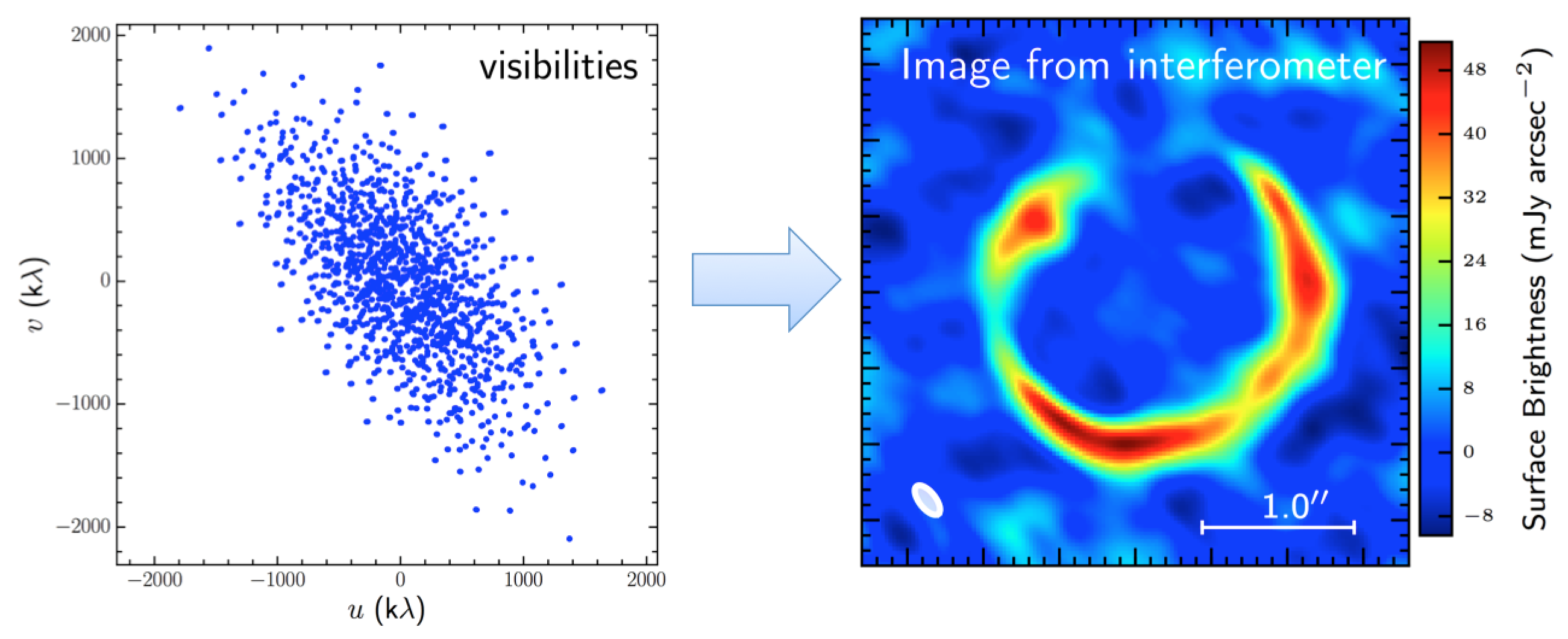
Lens modelling in the uv-plane

By looking at Fig. 3, it is clear that the lens modelling of interferometric images needs to be carried out in Fourier space in order to minimize the effect of correlated noise in the image domain and to properly account for the undersampling of the signal in Fourier space, which produces un-physical features in the reconstructed image.

We can still apply the regularised semi-linear inversion formalism with adaptive pixel scale described in Modelling of strongly lensed galaxies. The merit function is now defined using the visibility function as follows

(4) $\begin{eqnarray*} G_{\lambda} & = & \frac{1}{2} \sum_{u,v}^{N_{\rm vis}} \left| \frac{V_{\rm model}(u,v) - V_{\rm obs}(u,v)}{\sigma(u,v)} \right| ^{2} + \lambda \frac{1}{2}{\bf S}^{T}{\bf H}{\bf S} \\ & = & \frac{1}{2} \sum_{u,v}^{N_{\rm vis}} \left| \frac{V_{\rm model}^{\mathbb R}(u,v) - V^{\mathbb R}_{\rm obs}(u,v)}{\sigma(u,v)} \right| ^{2} \\ & ~ & + \frac{1}{2} \sum_{u,v}^{N_{\rm vis}} \left| \frac{V_{\rm model}^{\mathbb I}(u,v) - V^{\mathbb I}_{\rm obs}(u,v)}{\sigma(u,v)} \right| ^{2} \\ & ~ & + \lambda \frac{1}{2}{\bf S}^{T}{\bf H}{\bf S} \end{eqnarray*}$

where $N_{\rm vis}$ is the number of the observed visibilities $V_{\rm obs} = V_{\rm obs}^{\mathbb R} + i V_{\rm obs}^{\mathbb I}$ , while $\sigma^{2} = \sigma^{2}_{\mathbb R} + \sigma^{2}_{\mathbb I}$ , with $\sigma_{\mathbb R}$ and $\sigma_{\mathbb I}$ representing the 1 $\sigma$ uncertainty on the real and imaginary parts of $V_{\rm obs}$ , respectively. Please note that, with this definition of the merit function, I am implicitly assuming, for the lens modelling, what is usually referred to as a natural weighting scheme for the visibilities.

I can now introduce a rectangular matrix of complex elements $\hat{F}_{jk} = \hat{f}^{\mathbb R}_{jk} + \hat{f}^{\mathbb I}_{jk}$ , with $k = 1, .., N_{\rm vis}$ and $j = 1, .., N$ , $N$ being the number of pixels in the Source Plane (SP) considered in the modelling.

The term $\hat{f}_{jk}$ provides the Fourier transform of SP of value 1 at the $j$ -th pixel position and zero elsewhre, calculated at the location of the $k$ -th visibility point in the uv-plane. The effect of the primary beam is also accounted for in calculating $\hat{f}_{jk}$ .

Using the new introduced rectangular matrix, Eq.(5) can be re-written as

(5) $\begin{eqnarray*} G_{\lambda} & = & \frac{1}{2} \sum_{k=1}^{N_{\rm vis}} \left( \frac{\sum_{j=1}^{N}s_{j}\hat{f}^{\mathbb R}_{jk} - V_{{\rm obs},k}^{\mathbb R}}{\sigma_{k}} \right) ^{2} \\ & ~ & + \frac{1}{2} \sum_{k=1}^{N_{\rm vis}} \left( \frac{\sum_{j=1}^{N}s_{j}\hat{f}^{\mathbb I}_{jk} - V_{{\rm obs},k}^{\mathbb I}}{\sigma_{k}} \right) ^{2} \\ & ~ & + \lambda \frac{1}{2}{\bf S}^{T}{\bf H}{\bf S} \end{eqnarray*}$

If you now take the derivative of $G_{\lambda}$ with respect to $s_{i}$ and set it to 0 to find the minimum of the merit function you will discover that the solution can be express in matrix form

(6) $\begin{equation*} \boxed{{\bf S} = [{\bf \hat{F}} +\lambda {\bf H}]^{-1}\cdot{\bf \hat{D}}} \end{equation*}$

once you introduce the real matrixes

(7) $\begin{eqnarray*} \hat{\bf F}_{jk} & = & \sum_{l=1}^{N_{\rm vis}} \frac{\hat{f}_{jl}^{\mathbb R}\hat{f}_{lk}^{\mathbb R} + \hat{f}_{jl}^{\mathbb I}\hat{f}_{lk}^{\mathbb I}}{\sigma_{l}^{2}} \\ \hat{\bf D}_{j} & = & \sum_{l=1}^{N_{\rm vis}} \frac{\hat{f}_{jl}^{\mathbb R}V_{{\rm obs},l}^{\mathbb R} + \hat{f}_{jl}^{\mathbb I}V_{{\rm obs},l}^{\mathbb I}}{\sigma_{l}^{2}} \end{eqnarray*}$

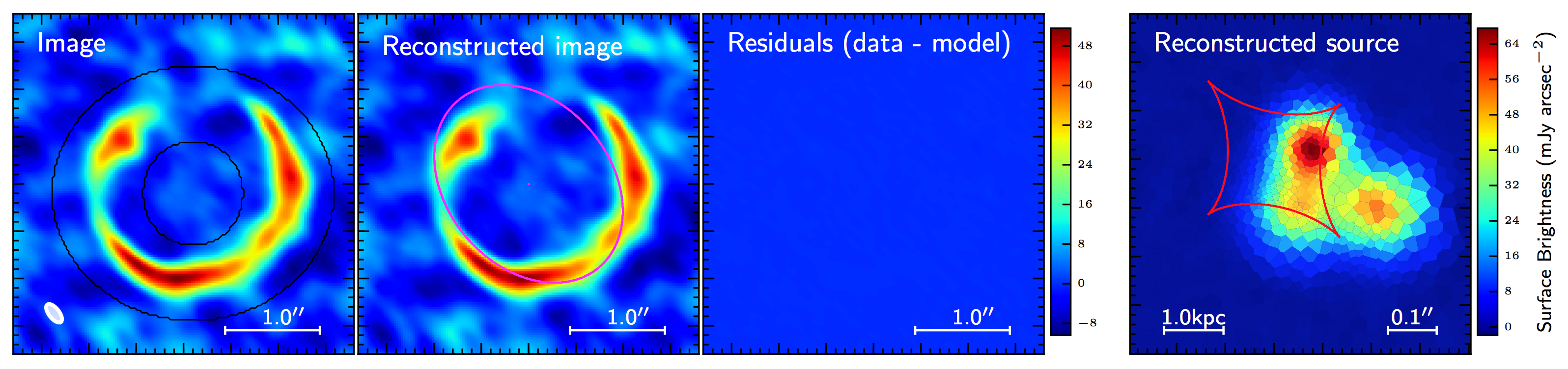
The regularization constant is computed using the exact same expression I provided for the modelling of imaging data, with, of course, $G_{\lambda}$ , ${\bf F}$ and $\sigma$ replaced by the corresponding quantities defined here. The definition of the regularization matrix, ${\bf H}$ , remains unchanged.

The result of the application of this formalism to the simulated image in Fig. 3 is shown in Fig. 4 below. As you can see the reconstructed source clearly shows the three distinct knots of emission, as expected.