There is a long literature on the modelling of strongly lensed galaxies. The approach I am going to describe here is based on few key papers: Warren & Dye 2003, Suyu et al. (2006), Nightingale & Dye (2015). The aim of the modelling is twofold:
1. Reconstructing the intrinsic light profile of the background source, i.e. how the source would look like if it hadn’t been gravitationally lensed;
2. Constraining the parameters that describe the mass distribution of the foreground object acting as the lens.
As I am mainly interested in exploiting gravitational lensing for studying the properties of distant galaxies, I will only focus on the first of the two points listed above, and thus assume that the mass distribution of the lens is known.
Simulated source
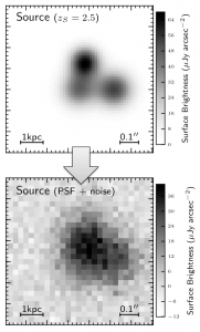
In order to explain how the source surface brightness can be reconstructed from its lensed images I am going to use the simple simulated source shown in the top panel panel of Fig. 1. It is made up of three spherical Gaussian profiles with different widths and normalisations. Clumpy sources are what we usually find when observing dusty star forming galaxies (DSFGs) at sub-mm/mm wavelengths, with clumps representing individual giant molecular clouds. If I place the source at redshift z∼2.5 – the median redshift of sub-mm selected DSFGs –, a physical scale of 1 kpc would subtend an angular scale of 0.17″. The simulated source extends over ~0.5″, with individual clumps thus having a physical size of few hundreds of pc, comparable to that expected for giant molecular clouds.
Figure 1. Simulated source
Let’s now assume that we observe this source with a telescope that can achieve a resolution of 0.15″. This is the value of the Full-Width at Half Maximum (FWHM) of the Point Spread Function (PSF) of the telescope. A value FWHM=0.15″ is comparable to that achievable in the near-infrared when using the Wide-Field Camera 3 (WFC3) onboard the Hubble space telescope. The bottom panel of Fig. 1 shows how that source would look like if imaged with such a telescope. In practise I have convolved the source with the PSF, rescaled the image to a pixel scale of 0.05″ (to ensure a good sampling of the PSF) and added some noise.
The source is clearly detected but only partially resolved: it does show an elongated structure but it is very hard to tell how many clumps it is made of and what their shape is.
Simulated lensed source
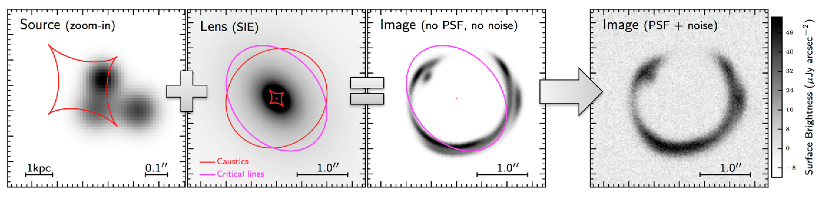
Now I am going to produce a gravitationally lensed version of the simulated source shown in the top panel of Fig. 1. In order to do that I need to specify a model for the mass distribution of the object acting as the lens, which will be located close to the line of sight of the observer to the source. The model will allow me to compute the path of the rays of light which are deflected by the lens towards the Earth. Observations seem to indicate that in most galaxy-scale lensing events the mass profile of foreground object, which is usually an elliptical galaxy, follows quite closely a Singular Isothermal Ellipsoid (SIE; Kormann, Schhneider & Bartelmann 1994) model (e.g. Barnabè et al. 2009). So this is the model I adopted here. I followed the formalism of Tessore & Metcalf (2015) to compute the lensing properties of the SIE profile, i.e. the deflection angle map, the magnification pattern, the caustics and the critical lines. The result is shown in the Fig. 2, third panel from the left. The right-hand panel in the same figure shows instead the lensed source after convolution with the PSF and with noise added (the level of the noise is the same I used in the bottom panel of Fig. 1).
Figure 2. Simulated lensed source
As you probably noticed, the emission from the lens is not shown in the simulated observation of the lensing event. In fact, I assumed that the foreground object acting as a lens has been already removed, by fitting its light profile with e.g. GALFIT and then subtracting it off.
Note that for high-spatial resolution observation performed in the sub-mm/mm you don’t usually need to care about subtracting the lens as nature does the job for you! In fact the lens is usually a passively evolving massive elliptical galaxy which contains only tiny amounts of dust (if any at all) and, therefore, its emission at sub-mm/mm wavelengths is barely detectable.
By looking at the simulated observation of the lensed galaxy you can tell that there is structure in the source. At least two sets of lensed images can be appreciated (particularly by those with a little bit of experience with gravitational lensing events). This is because gravitational lensing stretches the image of the source thus increasing the spatial resolution of the observations (recall the image of the lensed dog). It is this stretching that allows us to better probe the small scale structure in the background source. Such an effect will become clearer once I will reconstruct the source surface brightness from the observed lensed images.
Source reconstruction
Now that we have a simulated observation of a lensed galaxy we are left with the most important task: how to reconstruct the surface brightness of the background source from the observation of its lensed images. As I anticipated before, I will assume, for simplicity, that we know the mass distribution of the lens (its orientation angle, ellipticity, normalisation etc..). So we know the deflection angle map.
The naive approach to the source reconstruction is that of assuming an analytic profile for the source surface brightness, which will depend on a set of free parameters. For example, for an elliptical Sersic profile the free parameters would be 6: the coordinates of the centroid, the ellipticity, the rotation angle, the sersic index and the sersic half-light radius. The deflection angle map is then used to produce the lensed image of the source for any set of values of the free parameters. The image is compared, pixel by pixel, with the observed one via the merit function
(1)
where is the number of pixels in the image that are considered for the modelling, is the measured surface brightness at the th pixel position, with associated error , while is the predicted surface brigthness at the same pixel position. The set of parameters that minimize the merit function is the one that better describe the source surface brightness profile.
The problem with this approach is that you need to search a 6D parameter space for the source surface brightness profile alone. The dimension of the parameters space increases to 11 once you also minimise over the lens model parameters. Besides, it is not guarantee that the source can be described by a Sersic profile and/or that the source comprises just one knot of emission. Adding multiple profiles means increasing the parameter space, and, therefore, the risk of degeneracies in the solution.
A way to overcome this problems is to treat the background source as an ensemble of (not necessarily square) pixels without making any assumption on the profile of the source. Each pixel describes the surface brightness of the source at that position and is treated as a free parameter. You might think that this is madness: in fact, the background source may extend over hundreds of pixels. Does that mean that we have to search a parameter space with hundreds of dimensions?? The answer, of course, is no! It turns out that you can find an exact solution to the problem via a single matrix inversion. Let’s see how.
• Pixellated source: the Semi-Linear Inversion Method
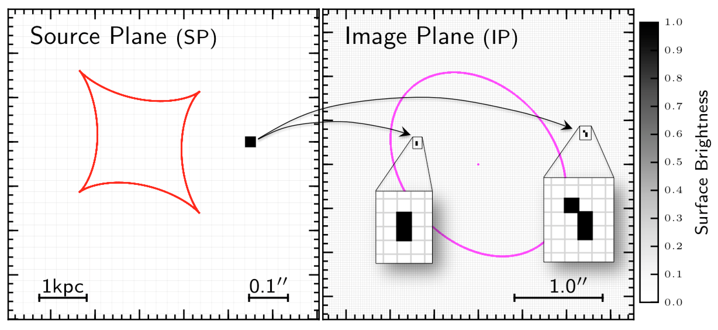
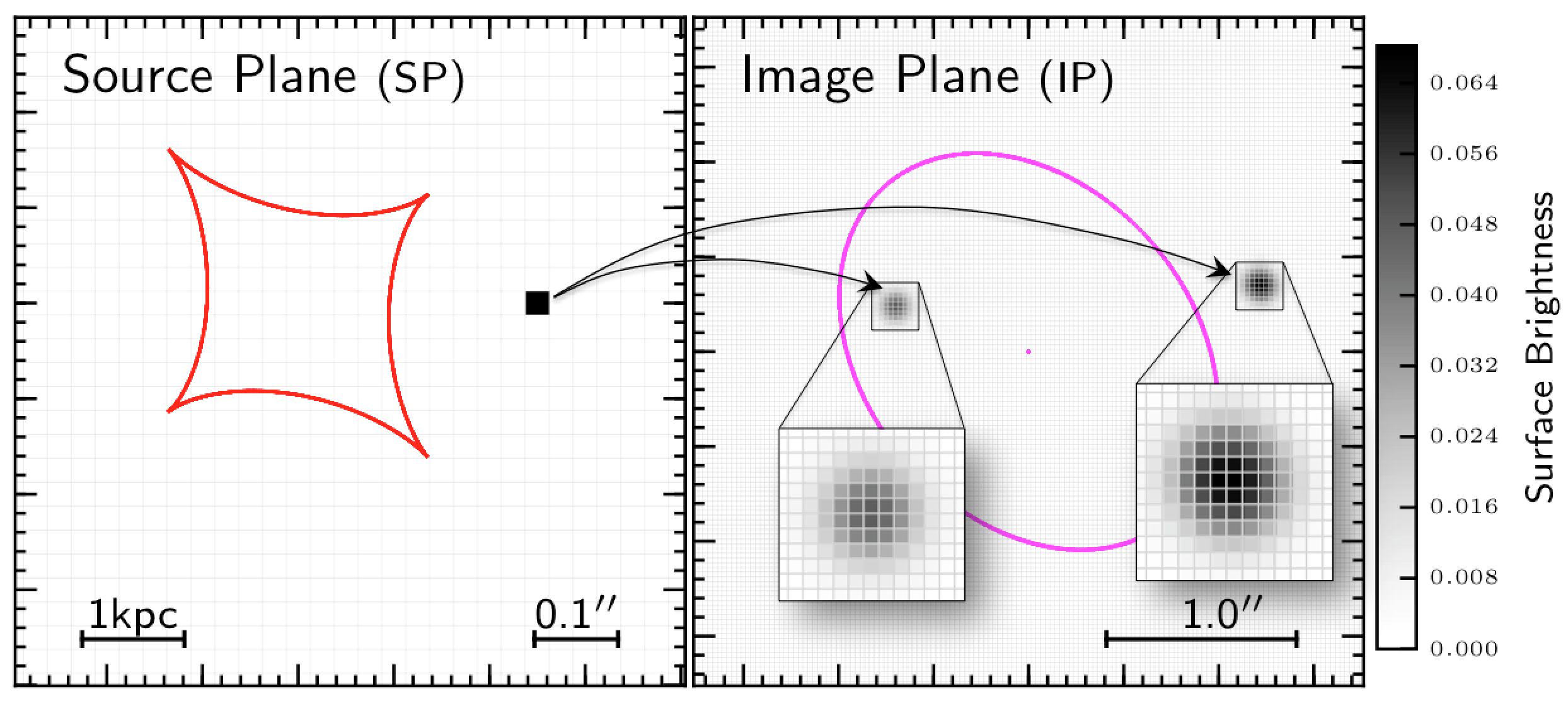
First of all let’s define two planes, both orthogonal to the line-of-sight of the observer to the lens: the source plane (SP), which contains the projected source surface brightness and the image plane (IP), where the lensed images of the source are formed. The two planes are represented in Fig. 3: the SP on the left and the IP on the right. Both are divided into squarepixels (0.05″ in size) whose values represent the surface brightness counts. In the IP, the pixels values are described by an array of elements , with , and associated statistical uncertainties , while in the SP the unknown surface brightness counts are represented by the array of elements , with .
Figure 3. Top-panels: One pixel, of unit value, in the Source Plane is lensed into 5 pixels in the Image Plane. Because gravitational lensing conserves the surface brightness, the 5 non-null pixels in the IP will also have unit value. Bottom-panels: the lensed image is convolved with the PSF. As a consequence the lensed images of the SP pixel are spread over many more pixels and their value is lower than 1.
In Fig. 3 I have highlighted one pixel in the SP which is then lensed into the IP. The mapping from the SP to the IP is defined by the adopted lens mass model and can be described by a matrix, whose element correspond to the surface brightness of the th pixel in the lensed and PSF-convolved image of source pixel held at unit surface brightness.
In practise, to construct the element you first create a SP with all pixel values set to 0, except for the th pixel which, instead, is set to 1 (this is exactly the case shown in Fig. 3). Then this SP is lensed into the IP (top-right panel in Fig. 3) and convolved with the PSF (bottom-right panel in Fig. 3); is the value of the th pixel in the resulting image. The matrix built in this way can be used to compute the value of the IP surface brightness, , at any pixel position , given the source surface brightness counts :
(2)
At this point the model image can be compared with the observed image via the merit function
(3)
The most likely solution is the one that minimises the merit function. By taking the derivative of with respect to one gets
(4)
Note the linear dependence of this expression on the parameters. Therefore finding the most likely source surface brightness distribution, for a fixed mass model, translates into solving a system of linear equations!
If we now define the following vectors:
Therefore the solution for the source surface brightness counts can be found via a simple matrix inversion
(8)
Of course this holds true for a fixed mass model. In general, the solution does not have a linear dependence on the lens model parameters, hence the name semi-linear inversion method. The final solution is achieved by sampling the lens parameters space, via e.g. a Monte Carlo Markov Chain (MCMC), and by using Eq. (8) to calculate, at each step, the solution for the source surface brightness and the corresponding value of the merit function, until the minimum of that function is found.
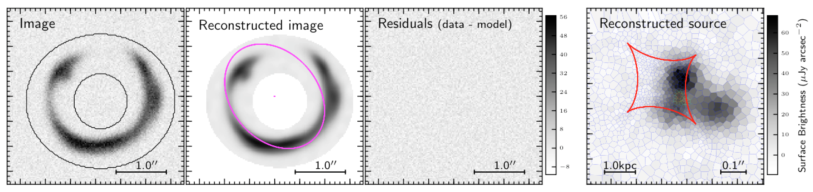
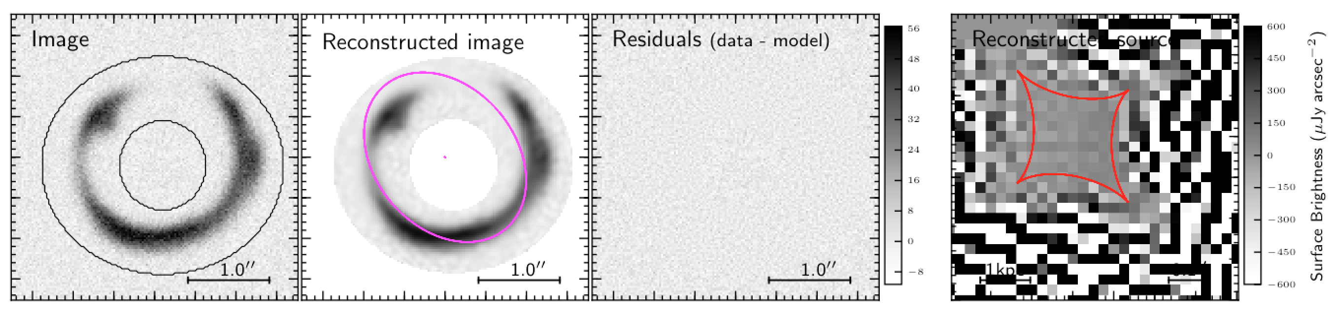
If we now apply Eq. (8) to the simulated observation of the lensed source in Fig. 2, we obtain the result shown in Fig. 4 below. In the left-hand panel is the simulated image, with the doughnut-like area marking the region considered for the definition of the merit function. In the second panel from the left is the reconstructed image, which looks pretty good, consistently with the residuals shown in the third panel. However the reconstructed source, in the right-hand panel, is noting close to what one would expect. It is actually very disappointing: An ensemble of chaotic pixel values! Why such a results?
In deriving the solution for the source surface brightness counts I have implicitly assumed that each SP pixel behaved independently from the others. As a consequence, the final solution shows severe discontinuities and pixel-to-pixel variations due to the noise in the image being modelled. The way to overcome this problem is to add a regularization term to the merit function as explained below.
Figure 4. Reconstructed source without regularisation term.
• Regularized solution
In order to obtain a solution for the source surface brightness that has a physical meaning we need to force a smooth variation in the value of nearby pixels in the SP. This is achieved by assuming a prior on the parameters , in the form of a regularization term , which is added to the merit function
(9)
where is a regularization constant, which controls the strength of the regularization and is the regularization matrix, with elements . The regularization term is chosen to have a linear dependence on the parameters in order to preserve the matrix formalism. In fact, it is easy to show that the minimum of the newly defined merit function satisfies the condition
(10)
and, therefore, the solution can still be derived via a matrix inversion
(11)
Bayesian analysis allows us to derive the value of the regularization constant that produced the most probable solution for . Assuming a constant prior on , its value is obtained by maximizing the Bayesian evidence (Suyu et al. 2006)
(12)
where represents here the set of values obtained from Eq. (11) for a given .
The regularized solution is shown in the right-hand panel of Fig. 5. Now the reconstructed source looks more like what we were expecting and if we compare this result with the simulated image of the un lensed source in the bottom panel of Fig. 1, we can definitely appreciate the magnifying power of gravitational lensing events: the source is now clearly resolved into 3 knots of emission, at variance with the unlensed case.
Figure 5. Reconstructed source with regularization and with square pixels.
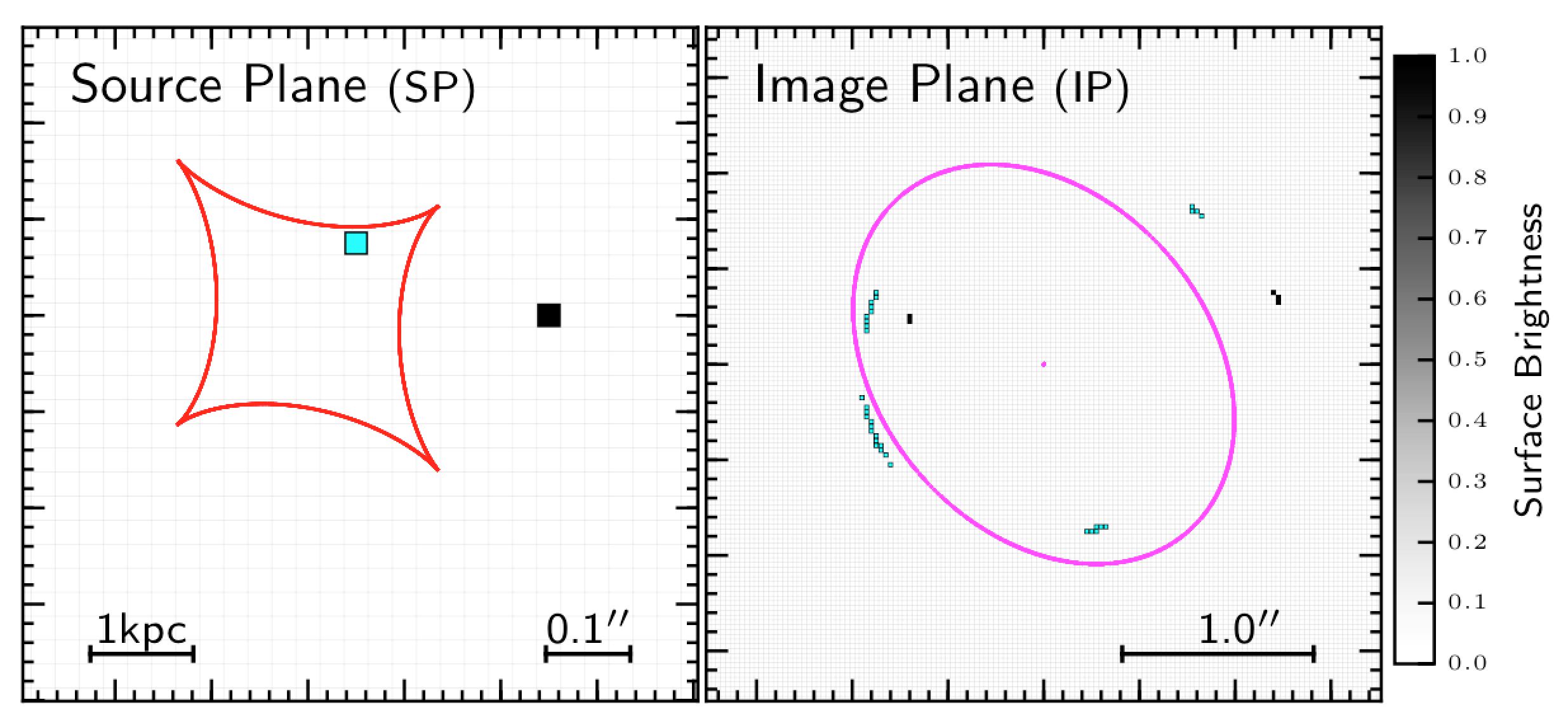
There is way in which we can further improve the source reconstruction. In fact, as illustrated in Fig. 6, the pixels in the SP that are closer to the lens caustics are multiply imaged over different regions in the IP, and therefore benefit from better constraints during the source reconstruction process, compared to pixels located further aways from the same lines. As a consequence, the noise in the reconstructed source surface brightness distribution significantly varies across the SP. At the same time, in highly magnified regions of the SP the information on the source properties at sub-pixel scales is not fully exploited. In order to overcome this issue a pixel with size that adapts to the magnification pattern can be adopted.
Figure 6. Pixels closer to the caustics (red curve) in the SP are lensed into a larger number of pixels in the IP compared to SP pixels that are farther away from the caustics
• Solution with adaptive pixel scale
An interesting SP pixellization scheme has been recently proposed by Nightingale & Dye (2015). For a fixed mass model the IP pixel centres are traced back to the SP and a k-means clustering algorithm is used to group them and to define new pixel centres in the SP. These centres are then used to generate Voronoi cells, mainly for visualization purposes. Within this adaptive pixelization scheme I have adopted a gradient regularization term defined as:
(13)
where are the counts members of the set of Voronoi cells that share at least one vertex with the th pixel.
The regularized solution with adaptive pixel scale is shown in the right-hand panel of Fig. 7 and it is definitely an improvement compared to the square pixel SP solution shown in Fig. 5, as the individual source components are now clearly distinguishable.
Figure 7. Reconstructed source with regularization and with adaptive pixel scale.

 is the number of pixels in the image that are considered for the modelling,
  is the measured surface brightness at the
  th pixel position, with associated error
  , while
  is the predicted surface brigthness at the same pixel position. The set of parameters that minimize the merit function is the one that better describe the source surface brightness profile.
 , and associated statistical uncertainties
  , with
  .
. 
 matrix, whose element
  correspond to the surface brightness of the
  held at unit surface brightness.

 with respect to
![\begin{eqnarray*} {\bf S} & = & [s_{1}, s_{2}, ... , s_{\mathcal{I}}] \nonumber \\ {\bf D} & = & \left[\sum_{j=1}^{\mathcal{J}}\frac{f_{1j}d_{j}}{\sigma_{j}^{2}}, \sum_{j=1}^{\mathcal{J}}\frac{f_{2j}d_{j}}{\sigma_{j}^{2}}, ... , \sum_{j=1}^{\mathcal{J}}\frac{f_{\mathcal{I}j}d_{j}}{\sigma_{j}^{2}} \right], \end{eqnarray*}](http://www.mattianegrello.com/wp-content/ql-cache/quicklatex.com-2f5c303102fa395d58326d2c6d6fc640_l3.png "Rendered by QuickLaTeX.com")
 with elements
![\begin{eqnarray*} [{\bf F}]_{ik} = F_{ik} = \sum_{j=1}^{\mathcal{J}}\frac{f_{ij}f_{kj}}{\sigma_{j}^{2}}, \end{eqnarray*}](http://www.mattianegrello.com/wp-content/ql-cache/quicklatex.com-705888c0ed40a481e13f9579e151edcb_l3.png "Rendered by QuickLaTeX.com")


 , which is added to the merit function
 is a regularization constant, which controls the strength of the regularization and
  is the regularization matrix, with elements
  . The regularization term is chosen to have a linear dependence on the parameters
 ![\begin{equation*} [{\bf F} + \lambda{\bf H}] \cdot {\bf S} = {\bf D}, \end{equation*}](http://www.mattianegrello.com/wp-content/ql-cache/quicklatex.com-5e6c6c52bb8e468d384d0df215488417_l3.png "Rendered by QuickLaTeX.com")
![\begin{equation*} \boxed{{\bf S} = [{\bf F} +\lambda {\bf H}]^{-1}\cdot{\bf D}} \end{equation*}](http://www.mattianegrello.com/wp-content/ql-cache/quicklatex.com-770c257a3f9f2a0f4785ff292777eab9_l3.png "Rendered by QuickLaTeX.com")
 . Assuming a constant prior on
  (Suyu et al. 2006)
![\begin{eqnarray*} 2\ln{[\epsilon(\lambda)]} &=& - G_{\lambda}({\bf S}) - \ln{[{\rm det}({\bf F} + \lambda {\bf H})]} \\ &~& + \ln{[{\rm det}(\lambda{\bf H})]} - \sum_{j=1}^{\mathcal J}\ln{(2\pi\sigma_{j}^{2})}, \end{eqnarray*}](http://www.mattianegrello.com/wp-content/ql-cache/quicklatex.com-aa941ab8bef99e285cdb1f32a6f4c28d_l3.png "Rendered by QuickLaTeX.com")
 represents here the set of
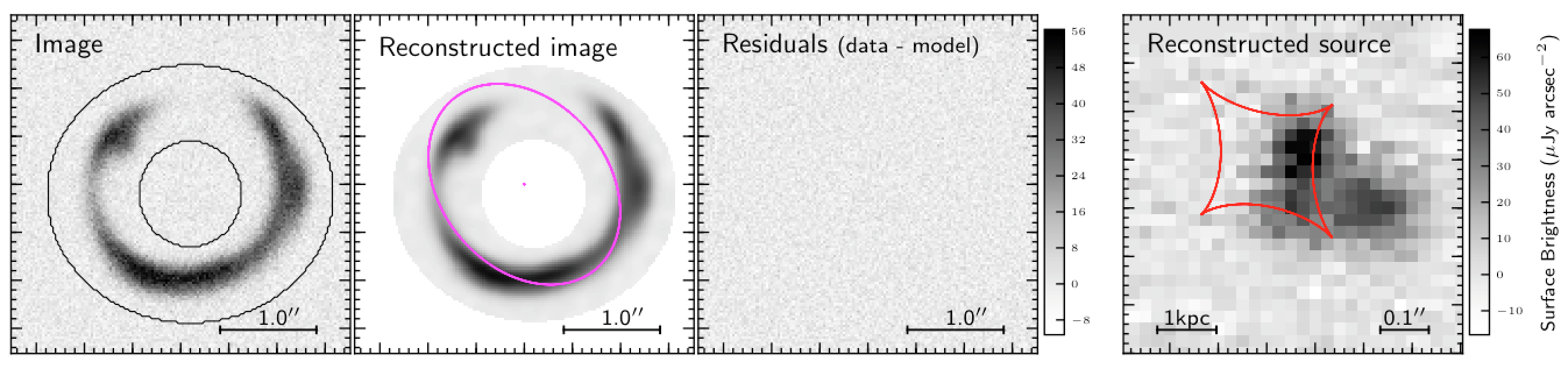

 are the counts members of the set of Voronoi cells that share at least one vertex with the